Prepare, transform, and orchestrate your data using AWS Glue DataBrew, AWS Glue ETL, and AWS Step Functions

Data volumes in organizations are increasing at an unprecedented rate, exploding from terabytes to petabytes and in some cases exabytes. As data volume increases, it attracts more and more users and applications to use the data in many different ways—sometime referred to as data gravity .

Source: Prepare, transform, and orchestrate your data using AWS Glue DataBrew, AWS Glue ETL, and AWS Step Functions

As data gravity increases, we need to find tools and services that allow us to prepare and process a large amount of data with ease to make it ready for consumption by a variety of applications and users. In this post, we look at how to use AWS Glue DataBrew and AWS Glue extract, transform, and load (ETL) along with AWS Step Functions to simplify the orchestration of a data preparation and transformation workflow.

DataBrew is a visual data preparation tool that exposes data in spreadsheet-like views to make it easy for data analysts and data scientists to enrich, clean, and normalize data to prepare it for analytics and machine learning (ML) without writing any line of code. With more than 250 pre-built transformations, it helps reduce the time it takes to prepare the data by about 80% compared to traditional data preparation approaches.

AWS Glue is a fully managed ETL service that makes it simple and cost-effective to categorize your data, clean it, enrich it, and move it reliably between various data stores and data streams. AWS Glue consists of a central metadata repository known as the AWS Glue Data Catalog, an ETL engine that automatically generates Python or Scala code, and a flexible scheduler that handles dependency resolution, job monitoring, and retries. AWS Glue is serverless, so there’s no infrastructure to set up or manage.

Step Functions is a serverless orchestration service that makes it is easy to build an application workflow by combining many different AWS services like AWS Glue, DataBrew, AWS Lambda, Amazon EMR, and more. Through the Step Functions graphical console, you see your application’s workflow as a series of event-driven steps. Step Functions is based on state machines and tasks. A state machine is a workflow, and a task is a state in a workflow that represents a single unit of work that another AWS service performs. Each step in a workflow is a state.

Overview of solution

DataBrew is a new service we introduced in AWS Re:invent 2020 in the self-serviced data preparation space and is focused on the data analyst, data scientist, and self-service audience. We understand that some organizations may have use cases where self-service data preparation needs to be integrated with a standard corporate data pipeline for advanced data transformation and operational reasons. This post provides a solution for customers who are looking for a mechanism to integrate data preparation done by analysts and scientists to the standard AWS Glue ETL pipeline using Step Functions. The following diagram illustrates this workflow.

Architecture overview

To demonstrate the solution, we prepare and transform the publicly available New Your Citi Bike trip data to analyze bike riding patterns. The dataset has the following attributes.

Field Name	Description
starttime	Start time of bike trip
stoptime	End time of bike trip
start_station_id	Station ID where bike trip started
start_station_name	Station name where bike trip started
start_station_latitude	Station latitude where bike trip started
start_station_longitude	Station longitude where bike trip started
end_station_id	Station ID where bike trip ended
end_station_name	Station name where bike trip ended
end_station_latitude	Station latitude where bike trip ended
end_station_longitude	Station longitude where bike trip ended
bikeid	ID of the bike used in bike trip
usertype	User type (customer = 24-hour pass or 3-day pass user; subscriber = annual member)
birth_year	Birth year of the user on bike trip
gender	Gender of the user (zero=unknown; 1=male; 2=female)

We use DataBrew to prepare and clean the most recent data and then use Step Functions for advanced transformation in AWS Glue ETL.

For the DataBrew steps, we clean up the dataset and remove invalid trips where either the start time or stop time is missing, or the rider’s gender isn’t specified.

After DataBrew prepares the data, we use AWS Glue ETL tasks to add a new column tripduration and populate it with values by subtracting starttime from endtime.

After we perform the ETL transforms and store the data in our Amazon Simple Storage Service (Amazon S3) target location, we use Amazon Athena to run interactive queries on the data to find the most used bikes to schedule maintenance, and the start stations with the most trips to make sure enough bikes are available at these stations.

We also create an interactive dashboard using Amazon QuickSight to gain insights and visualize the data to compare trip count by different rider age groups and user type.

The following diagram shows our solution architecture.

Prerequisites

To follow along with this walkthrough, you must have an AWS account. Your account should have permission to run an AWS CloudFormation script to create the services mentioned in solution architecture.

Your AWS account should also have an active subscription to QuickSight to create the visualization on processed data. If you don’t have a Quicksight account, you can sign up for an account.

Create the required infrastructure using AWS CloudFormation

To get started, complete the following steps:

1. Choose Launch Stack to launch the CloudFormation stack to configure the required resources in your AWS account.
   
2. On the Create stack page, choose Next.
   
3. On the Specify stack details page, enter values for Stack name and Parameters, and choose Next.
   
4. Follow the remaining instructions using all the defaults and complete the stack creation.

The CloudFormation stack takes approximately 2 minutes to complete.

5. When the stack is in the CREATE_COMPLETE state, go to the Resources tab of the stack and verify that you have 18 new resources.
   

In the following sections, we go into more detail of a few of these resources.

Source data and script files S3 bucket

The stack created an S3 bucket with the name formatted as <Stack name>-<SolutionS3BucketNameSuffix>.

On the Amazon S3 console, verify the creation of the bucket with the following folders:

• scripts – Contains the Python script for the ETL job to process the cleaned data
• source – Has the source City Bike data to be processed by DataBrew and the ETL job

DataBrew dataset, project, recipe, and job

The CloudFormation stack also created the DataBrew dataset, project, recipe, and job for the solution. Complete the following steps to verify that these resources are available:

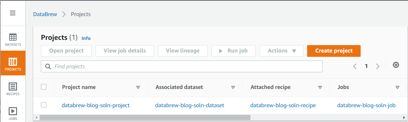
1. On the DataBrew console, choose Projects to see the list of projects.

You should see a new project, associated dataset, attached recipe, and job in the Projects list.

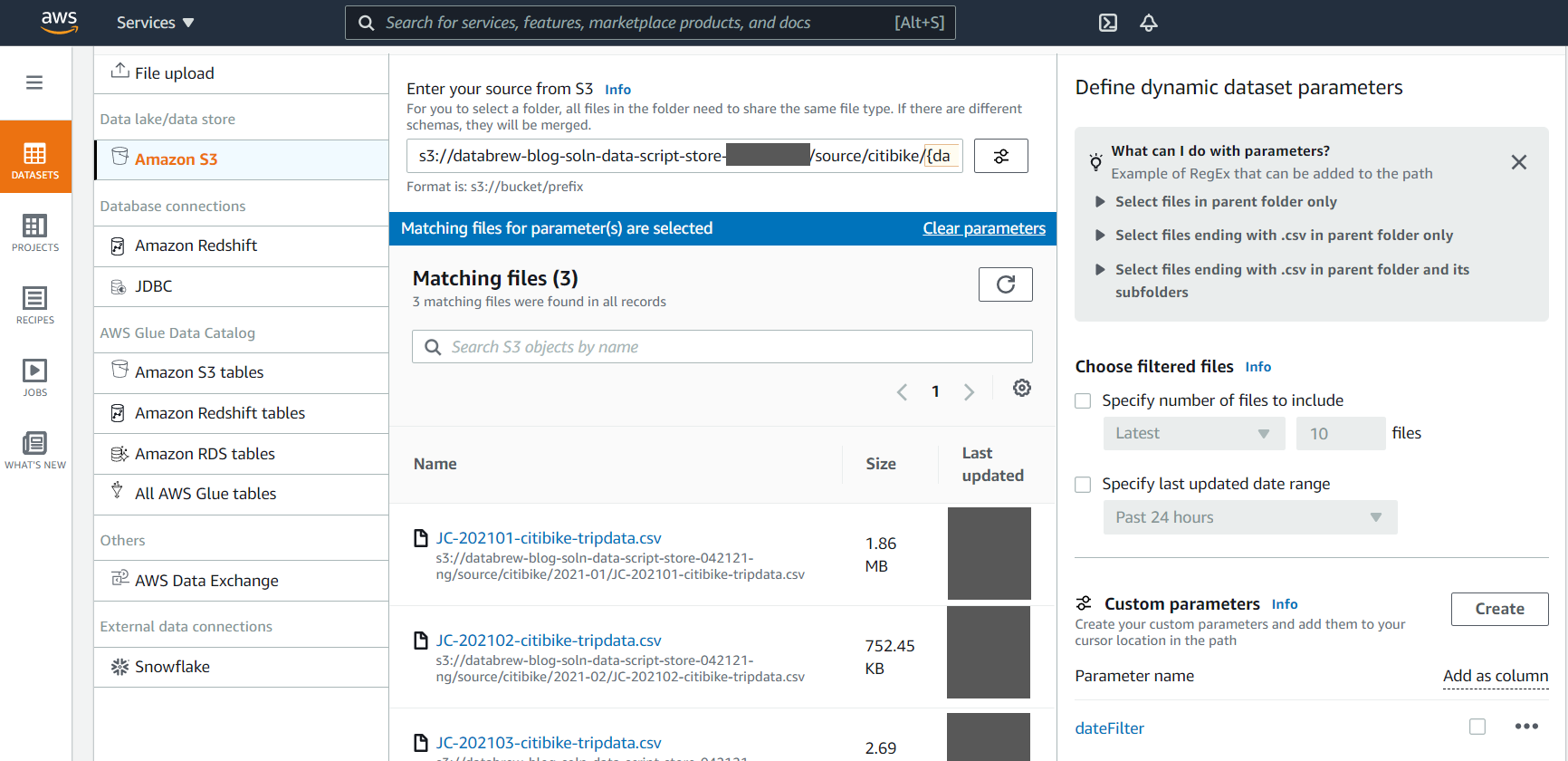
2. To review the source data, choose the dataset, and choose View dataset on the resulting popup.

You’re redirected to the Dataset preview page.

DataBrew lets you create a dynamic dataset using custom parameter and conditions. This feature helps you automatically process the latest files available in your S3 buckets with a user-friendly interface. For example, you can choose the latest 10 files or files that are created in the last 24 hours that match specific conditions to be automatically included in your dynamic dataset.

3. Choose the Data profile overview tab to examine and collect summaries of statistics about your data by running the data profile.
   
4. Choose Run data profile to create and run a profile job.
5. Follow the instructions to create and run the job to profile the source data.

The job takes 2–3 minutes to complete.

When the profiling job is complete, you should see Summary, Correlations, Value distribution, and Column Summary sections with more insight statistics about the data, including data quality, on the Data profile overview tab.

6. Choose the Column statistics tab to see more detailed statistics on individual data columns.

DataBrew provides a user-friendly way to prepare, profile, and visualize the lineage of the data. Appendix A at the end of this post provides details on some of the widely used data profiling and statistical features provided by DataBrew out of the box.

7. Choose the Data Lineage tab to see the information on data lineage.
   
8. Choose PROJECTS in the navigation pane and choose the project name to review the data in the project and the transformation applied through the recipe.

DataBrew provides over 250 transforms functions to prepare and transform the dataset. Appendix B at the end of this post reviews some of the most commonly used transformations.

We don’t need to run the DataBrew job manually—we trigger it using a Step Function state machine in subsequent steps.

AWS Glue ETL job

The CloudFormation stack also created an AWS Glue ETL job for the solution. Complete the following steps to review the ETL job:

1. On the AWS Glue console, choose Jobs in the navigation pane to see the new ETL job.
   
2. Select the job and on the Script tab, choose Edit script to inspect the Python script for the job.
   

We don’t need to run the ETL job manually—we trigger it using a Step Function state machine in subsequent steps.

Start the Step Function state machine

The CloudFormation stack created a Step Functions state machine to orchestrate running the DataBrew job and AWS Glue ETL job. A Lambda function starts the state machine whenever the daily data files are uploaded into the source data folder of the S3 bucket. For this post, we start the state machine manually.

1. On the Step Functions console, choose State machines in the navigation pane to see the list of state machines.
   
2. Choose the state machine to see the state machine details.
3. Choose Start execution to run the state machine.
   

The details of the state machine run are displayed on the Details tab.

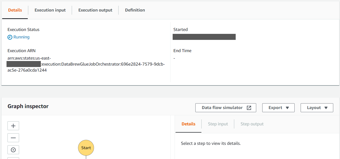
4. Review the Graph inspector section to observe the different states of the state machine. As each step completes, it turns green.
   
5. Choose the Definition tab to review the definition of the state machine.
   

When the state machine is complete, it should have run the DataBrew job to clean the data and the AWS Glue ETL job to process the cleaned data.

The DataBrew job removed all trips in the source dataset with missing starttime and stoptime, and unspecified gender. It also copied the cleaned data to the cleaned folder of the S3 bucket. We review the cleaned data in subsequent steps with Athena.

The ETL job processed the data in the cleaned folder to add a calculated column tripduration, which is calculated by subtracting the starttime from the stoptime. It also converted the processed data into columnar format (Parquet), which is more optimized for analytical processing, and copied it to the processed folder. We review the processed data in subsequent steps with Athena and also use it with QuickSight to get some insight into rider behavior.

Run an AWS Glue crawler to create tables in the Data Catalog

The CloudFormation stack also added three AWS Glue crawlers to crawl through the data stored in the source, cleaned, and processed folders. A crawler can crawl multiple data stores in a single run. Upon completion, the crawler creates or updates one or more tables in your Data Catalog. Complete the following steps to run these crawlers to create AWS Glue tables for the date in each of the S3 folders.

1. On the AWS Glue console, choose Crawlers in the navigation pane to see the list of crawlers created by the CloudFormation stack.If you have AWS Lake Formation enabled in the Region in which you’re implementing this solution, you may get insufficient lake formation permissions error. Please follow steps in Appendix C to provide required permission to the IAM role used by Glue Crawler to create table in citibike database.
   
2. Select each crawler one by one and choose Run crawler.
   

After the crawlers successfully run, you should see one table added by each crawler.

We run crawlers manually in this post, but you can trigger the crawlers whenever a new file is added to their respective S3 bucket folder.

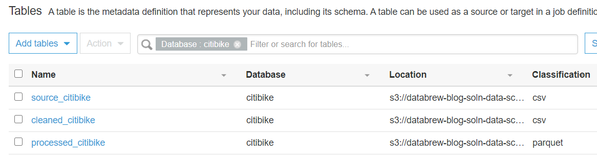
3. To verify the AWS Glue database citibike, created by the CloudFormation script, choose Databases in the navigation pane.
   
4. Select the citibike database and choose View tables.
   

You should now see the three tables created by the crawlers.

Use Athena to run analytics queries

In the following steps, we use Athena for ad-hoc analytics queries on the cleaned and processed data in the processed_citibike table of the Data Catalog. For this post, we find the 20 most used bikes to schedule maintenance for them, and find the top 20 start stations with the most trips to make sure enough bikes are available at these stations.

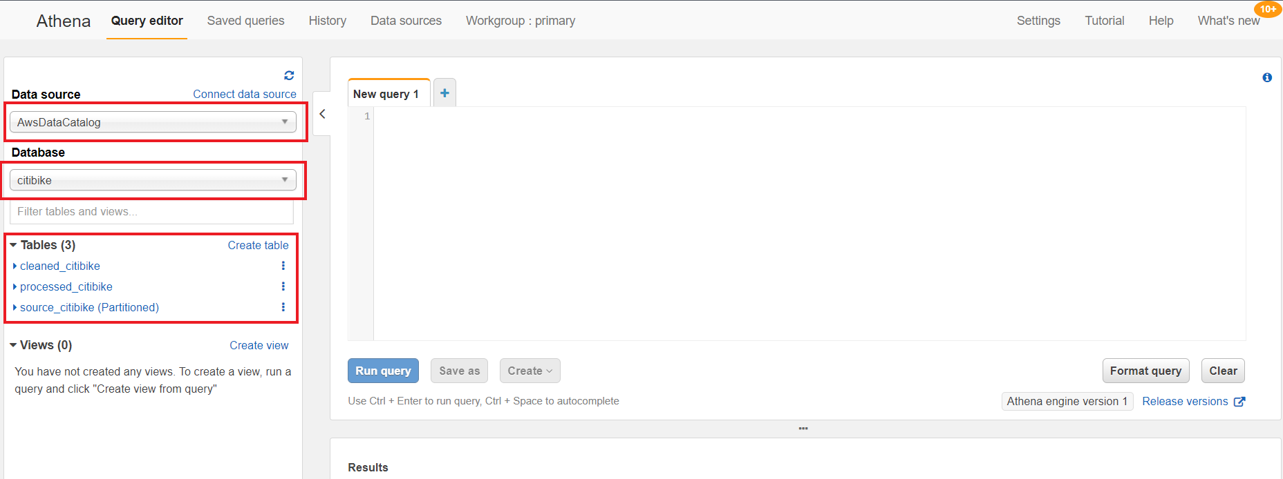
1. On the Athena console, for Data source, choose AwsDataCatalog.
2. For Database, choose citibike.

The three new tables are listed under Tables.

If you haven’t used Athena before in your account, you receive a message to set up a query result location for Athena to store the results of queries.

3. Run the following query on the New query1 tab to find the find the 20 most used bikes:

SELECT bikeid as BikeID, count(*) TripCount FROM "citibike"."processed_citibike" group by bikeid order by 2 desc limit 20;

If you have AWS Lake Formation enabled in the Region in which you’re implementing this solution, you may get error (similar to below error) in executing queries. To resolve the permission issues, please follow steps in Appendix D to provide “Select” permission to all tables in citibike database to logged in user using Lake Formation.

4. Run the following query on the New query1 tab to find the top 20 start stations with the most trips:

SELECT start_station_name, count(*) trip_count FROM "citibike"."processed_citibike" group by start_station_name order by 2 desc limit 20;

Visualize the processed data on a QuickSight dashboard

As the final step, we visualize the following data using a QuickSight dashboard:

• Compare trip count by different rider age groups
• Compare trip count by user type (customer = 24-hour pass or 3-day pass user; subscriber = annual member)

Your AWS account should also have an active subscription to QuickSight to create the visualization on processed data. If you don’t have a Quicksight account, you can sign up for an account.

1. On the QuickSight console, create a dataset with Athena as your data source.
   
2. Follow the instructions to complete your dataset creation.
   
3. Add a calculated filed rider_age using following formula:

dateDiff(parseDate({birth_year},"YYYY"), truncDate( "YYYY", now() ) ,"YYYY")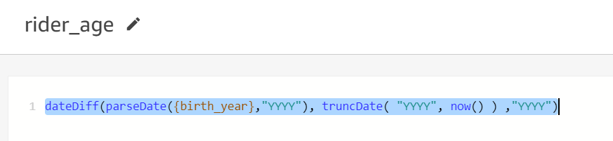

Your dataset should look like the following screenshot.

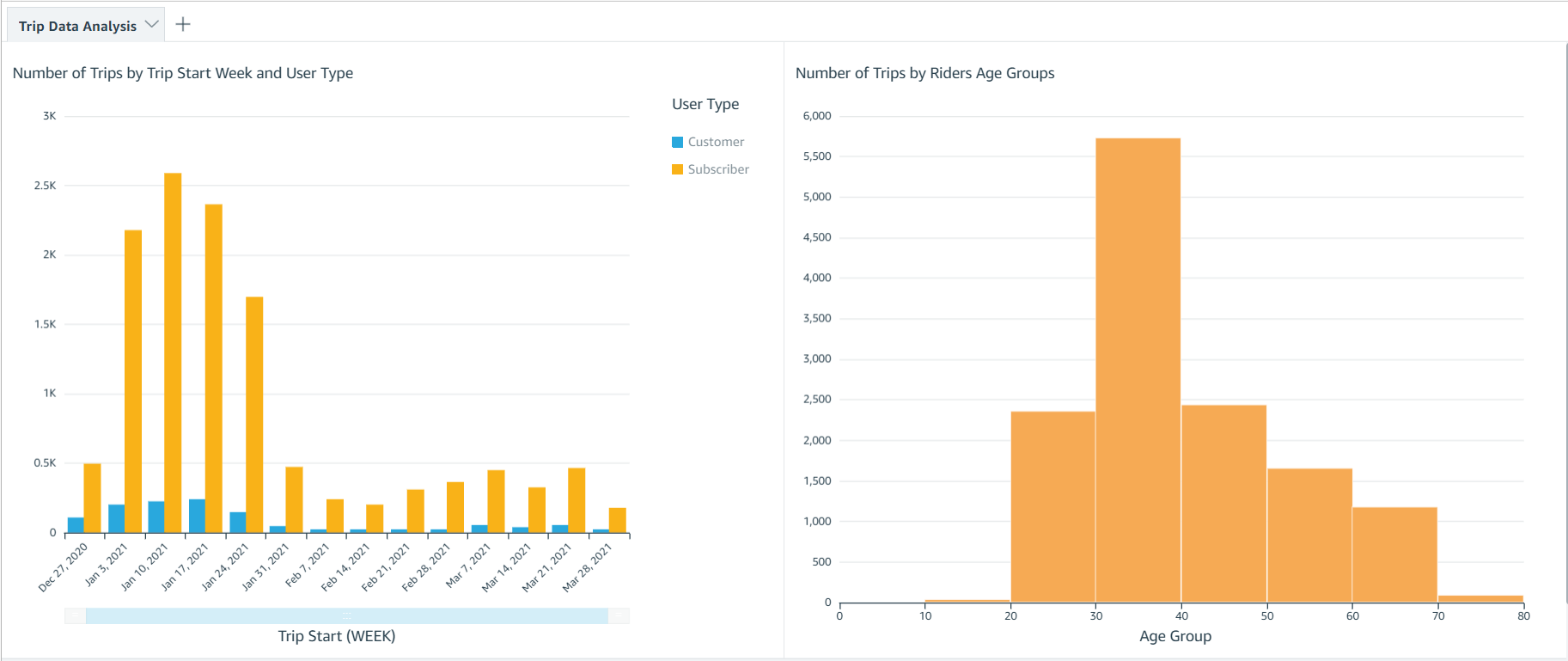
Now you can create visualizations to compare weekly trip count by user type and total trip count by rider age group.

Clean up

To avoid incurring future charges, delete the resources created for the solution.

1. Delete the DataBrew profile job created for profiling the source data.
   
2. Delete the CloudFormation stack to delete all the resources created by the stack.
   

Conclusion

In this post, we discussed how to use DataBrew to prepare your data and then further process the data using AWS Glue ETL to integrate it in a standard operational ETL flow to gather insights from your data.

We also walked through how you can use Athena to perform SQL analysis on the dataset and visualize and create business intelligence reports through QuickSight.

We hope this post provides a good starting point for you to orchestrate your DataBrew job with your existing or new data processing ETL pipelines.

For more details on using DataBrew with Step Functions, see Manage AWS Glue DataBrew Jobs with Step Functions.

For more information on DataBrew jobs, see Creating, running, and scheduling AWS Glue DataBrew jobs.

Appendix A

The following table lists the widely used data profiling and statistical features provided by DataBrew out of the box.

Type	Data type of the column
missingValuesCount	The number of missing values. Null and empty strings are considered as missing.
distinctValuesCount	The number of the value appears at least once.
entropy	A measure of the randomness in the information being processed. The higher the entropy, the harder it is to draw any conclusions from that information.
mostCommonValues	A list of the top 50 most common values.
mode	The value that appears most often in the column.
min/max/range	The minimum, maximum, and range values in the column.
mean	The mean or average value of the column.
kurtosis	A measure of whether the data is heavy-tailed or light-tailed relative to a normal distribution. A dataset with high kurtosis has more outliers compared to a dataset with low kurtosis.
skewness	A measure of the asymmetry of the probability distribution of a real-valued random variable about its mean.
Correlation	The Pearson correlation coefficient. This is a measure if one column’s values correlate to values of another column.
Percentile95	The element in the list that represents the 95th percentile (95% of numbers fall below this and 5% of numbers fall above it).
interquartileRange	The range between the 25th percentile and 75th percentile of numbers.
standardDeviation	The unbiased sample standard deviation of values in the column.
min/max Values	A list of the five minimum and maximum values in a column.
zScoreOutliersSample	A list of the top 50 outliers that have the largest or smallest Z-score. -/+3 is the default threshold.
valueDistribution	The measure of the distribution of values by range.

Appendix B

DataBrew provides the ability to prepare and transform your dataset using over 250 transforms. In this section, we discuss some of the most commonly used transformations:

• Combine datasets – You can combine datasets in the following ways:
  • Join – Combine several datasets by joining them with other datasets using a join type like inner join, outer join, or excluding join.
  • Union operation – Combine several datasets using a union operation.
  • Multiple files for input datasets – While creating a dataset, you can use a parameterized Amazon S3 path or a dynamic parameter and select multiple files.
• Aggregate data – You can aggregate the dataset using a group by clause and use standard and advanced aggregation functions like Sum, Count, Min, Max, mode, standard deviation, variance, skewness, kurtosis, as well as cumulative functions like cumulative sum and cumulative count.
• Pivot a dataset – You can pivot the dataset in the following ways:
  • Pivot operation – Convert all rows to columns.
  • Unpivot operation – Convert all columns to rows.
  • Transpose operation – Convert all selected rows to columns and columns to rows.
• Unnest top level value – You can extract values from arrays into rows and columns into rows. This only operates on top-level values.
• Outlier detection and handling – This transformation works with outliers in your data and performs advanced transformations on them like flag outliers, rescale outliers, and replace or remover outliers. You can use several strategies like ZScore, modified Z-score, and interquartile range (IQR) to detect outliers.
• Delete duplicate values – You can delete any row that is an exact match to an earlier row in the dataset.
• Handle or impute missing values – You have the following options:
  • Remove invalid records – Delete an entire row if an invalid value is encountered in a column of that row.
  • Replace missing values – Replace missing values with custom values, most frequent value, last valid value, or numeric aggregate values.
• Filter data – You can filter the dataset based on a custom condition, validity of a column, or missing values.
• Split or merge columns – You can split a column into multiple columns based on a custom delimiter, or merge multiple columns into a single column.
• Create columns based on functions –You can create new columns using different functions like mathematical functions, aggregated functions, date functions, text functions, windows functions like next and previous, and rolling aggregation functions like rolling sum, rolling count, and rolling mean.

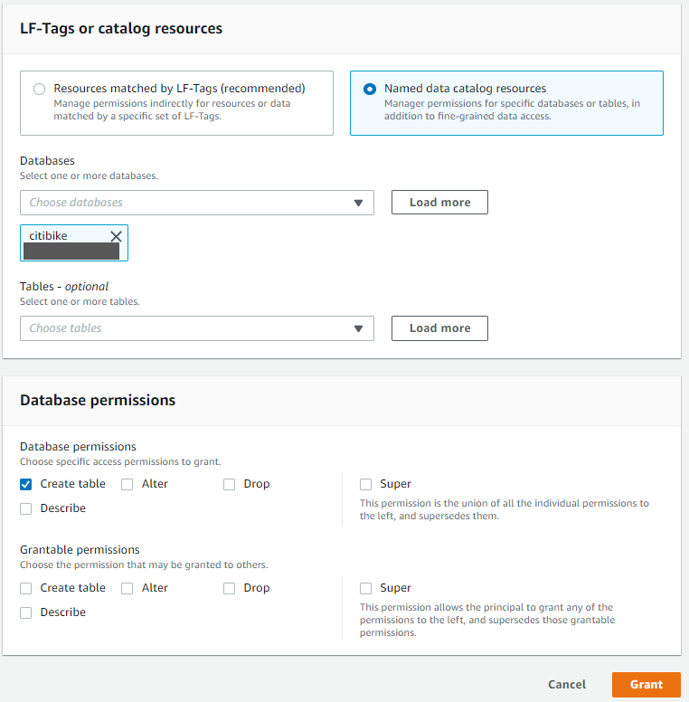
Appendix C

If you have AWS Lake Formation enabled in the Region in which you’re implementing this solution, you may get insufficient lake formation permissions error during Glue Crawler run.

Please provide create table permission in GlueDatabase (citibike) to GlueCrawlersRole (find the ARN from the Cloud Formation Resource section) for the crawler to create required table.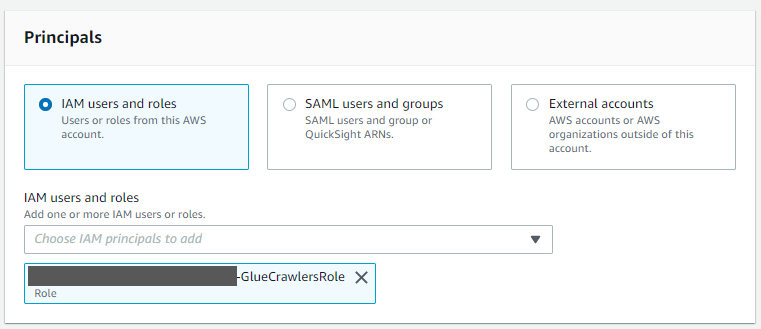

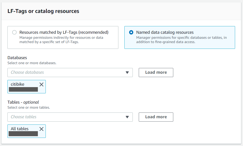
Appendix D

If you have AWS Lake Formation enabled in the Region in which you’re implementing this solution, you may get error similar to below error in running queries on tables in citibike database.

Please provide “Select” permission to all tables in GlueDatabase (citibike) to logged in user in Lake formation to allow the select on tables created by the solution to logged in user.

Original Post>

---

About the Authors

Narendra Gupta is a solutions architect at AWS, helping customers on their cloud journey with focus on AWS analytics services. Outside of work, Narendra enjoys learning new technologies, watching movies, and visiting new places.

Durga Mishra is a solutions architect at AWS. Outside of work, Durga enjoys spending time with family and loves to hike on Appalachian trails and spend time in nature.

Jay Palaniappan is a Sr. Analytics Specialist Solutions architect at AWS, helping media & entertainment customers adopt and run AWS Analytics services.