The key components of the Multi-Layer Perceptron architecture are:

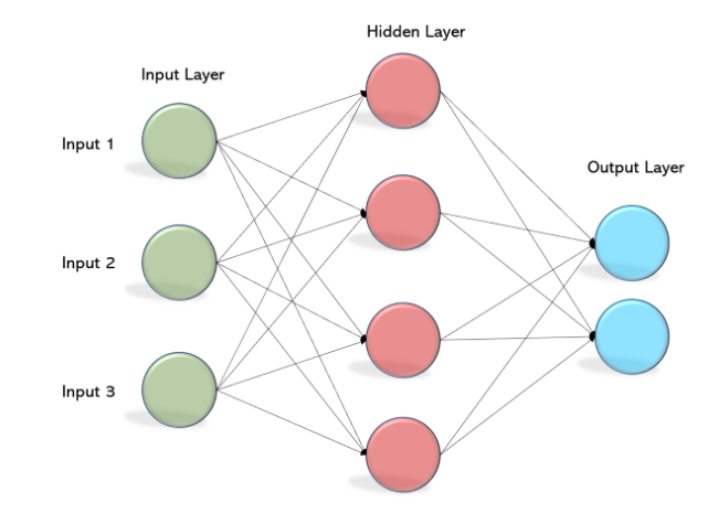
Input Layer:

• The initial layer, known as the input layer, receives the raw data or features.
• Each node in this layer represents a specific feature, forming the input vector.

Hidden Layers:

• Between the input and output layers, hidden layers process and transform the input data.
• Neurons within these layers apply weights and activation functions, allowing the network to capture intricate patterns and relationships.

Output Layer:

• The final layer, the output layer, produces the model’s predictions or classifications.
• The number of nodes in this layer depends on the nature of the task — one node for binary classification, multiple nodes for multi-class classification.

Each of the nodes of the layers described can be understood as individual perceptrons and have the usual components as showed in the previous article (weights, biases and activation functions).

The training process consists of the following steps:

Forward Propagation:

Also known as feedforward, in this step the input data is “fed” through the network, layer by layer, producing an output.

Backward Propagation:

• The network’s output is compared to the actual target, and the error is calculated.
• This error is then propagated backward through the network using optimization algorithms like gradient descent.
• Weights and biases are adjusted iteratively to minimize the error, enhancing the model’s performance.

Now, let’s dive into each step of the training process of the MLP and implement (in python) their key components.

Our MLP

For simplicity, in our example we’ll use a MLP with a input layer with 2 nodes, one single hidden layer with 3 nodes and a output layer with 1 node, as shown in figure below:

Simple MLP.

Without further ado, let’s start coding by importing necessary packages and declaring the key components:

import numpy as np

# Example usage:
input_size = 2
hidden_size = 3
output_size = 1

# initialize weights matrix and biases with random values
input_data = [[1,2], [3,4], [5,6]]
target = np.array([[3], [6], [9]])
input_data = np.array(input_data)

W_input_hidden = np.random.rand(hidden_size, input_size)
b_input_hidden = np.random.rand(hidden_size, 1)
W_hidden_output = np.random.rand(output_size, hidden_size)
b_idden_output = p.random.rand(output_size, 1)

With our input data, weights and biases, let’s pass the data through the layers using the sigmoid function as activation function and compare the output with the target values:

hidden_layer_input = W_input_hidden.dot(input_data.T) + b_input_hidden

array([[0.94267816, 0.99752498, 0.99989877],
 [0.96790071, 0.99904069, 0.9999722 ],
 [0.94229868, 0.99758374, 0.9999042 ]])

As we can see, the output is a matrix with 3 rows(one for each input entry) and 3 columns (one for each node of the hidden layer).

hidden_layer_output = sigmoid(hidden_layer_input)

array([[0.83389203, 0.96825381, 0.99463232],
 [0.94957477, 0.996385 , 0.99975218],
 [0.95051374, 0.99835873, 0.99994809]])

Now the output of the hidden layer will be the input of the output layer:

output_layer_input = W_hidden_output.dot(hidden_layer_output) + b_hidden_output

array([[1.01296163, 1.06912515, 1.07344231]])

That way, we now have a matrix with 1 row (the dimension of the output) and 3 columns (corresponding to the hidden layer size).

Finally, the output will be:

output = sigmoid(output_layer_input)

array([[0.73359934, 0.74443051, 0.745251]])

The output is too far from the target values (3, 6, 9), hence it’s necessary to train the MLP in order to get as close to the target values as possible.

In order to minimize the distance to the target values, we’ll use the Gradient Descent algorithm.

Gradient descent is an optimization algorithm used to minimize the loss function of a neural network, which measures the difference between the predicted outputs and the actual targets.

The basic idea is to iteratively adjust the parameters (weights and biases) of the MLP in the direction that reduces the loss, thereby improving the model’s performance.

In order to achieve that, we must update the weights and biases in the opposite direction of the gradient of the error of each layer relative to the weights and biases of the layer.

I’ll not bore the reader with the demonstration of the gradient of multivariate functions, so it’s enough to say that the gradient of the loss function relative to its parameters is:

gradient formula

where:

• d(ypred): derivative of the activation function (sigmoid function)

derivative of the sigmoid function.

• e: difference between target value and predicted
• lr: learning rate

In order to obtain the error of the previous layer (hidden layer), we must multiply the gradient with the output of the layer.

error of hidden layer.

where the matrix H is the matrix of weights and bias of the hidden layer.

Implementation in python:

 def d_sigmoid(x):
 return x * (1 - x)

lr = 0.01

# gradient of output layer
output_error = target - output
output_grad = d_sigmoid(output)*output_error*lr

# gradient of hidden layer
hidden_error = np.dot(output_grad, W_hidden_output.T)
hidden_grad = hidden_error * d_sigmoid(hidden_layer_output)*lr

# Update weights and biases using gradient descent
W_hidden_output += np.dot(output_grad, output_layer_input.T)
b_hidden_output += np.sum(output_grad)

W_input_hidden += np.dot(hidden_grad, input_data)
b_input_hidden += np.sum(hidden_grad, axis=0, keepdims=True)

That process will be performed iteratively for a number of epochs in order to train the MLP improving its performance.

Now we’ll create a MLP class to generalize the solution to any input and target data:

class MLP:
 def __init__(self, input_size, hidden_size, output_size):
 self.input_size = input_size
 self.hidden_size = hidden_size
 self.output_size = output_size

 # initialize weights matrix and biases
 self.W_input_hidden = np.random.rand(self.input_size, self.hidden_size)
 self.b_input_hidden = np.zeros((1, self.hidden_size))
 self.W_hidden_output = np.random.rand(self.hidden_size, self.output_size)
 self.b_hidden_output = np.zeros((1, self.output_size))

 # auxiliar functions

 def sigmoid(self, x):
 return 1 / (1 + np.exp(-x))

 def d_sigmoid(self, x):
 return x * (1 - x)

 def forward(self, input_data):
 hidden_layer_input = np.dot(input_data, self.W_input_hidden) + self.b_input_hidden
 hidden_layer_output = self.sigmoid(hidden_layer_input)
 output_layer_input = np.dot(hidden_layer_output, self.W_hidden_output) + self.b_hidden_output
 output = self.sigmoid(output_layer_input)

 return hidden_layer_output, output

 def backward(self, input_data, target, hidden_output, output, lr=0.2):

 # Backward propagation
 output_error = target - output
 output_grad = output_error * self.d_sigmoid(output)

 hidden_error = np.dot(output_grad, self.W_hidden_output.T)
 hidden_grad = hidden_error * self.d_sigmoid(hidden_output)

 # Update weights and biases using gradient descent
 self.W_hidden_output = self.W_hidden_output + np.dot(hidden_output.T, output_grad)*lr
 self.b_hidden_output = self.b_hidden_output + np.sum(output_grad)*lr

 self.W_input_hidden = self.W_input_hidden + np.dot(input_data.T, hidden_grad)*lr
 self.b_input_hidden = self.b_input_hidden + np.sum(hidden_grad, axis=0, keepdims=True)*lr

 def train(self, input_data, target, epochs=1000):
 for epoch in range(epochs):
 hidden_output, output = self.forward(input_data)
 self.backward(input_data, target, hidden_output, output)

• Applying to a real case (XOR gate)

Finally, we’ll use our MLP implementation to real data. For our example, let’s create a model that functions as a XOR gate.

As discussed earlier, a single perceptron is not able to solve non-linear problems such as the XOR gate, but a combination of perceptrons might do the trick.

XOR truth table (source: https://www.build-electronic-circuits.com/xor-gate/).

Let’s create the MLP and train it

# XOR truth table values
xor_input = np.array([[0, 0], [0, 1], [1, 0], [1, 1]])
xor_target = np.array([[0], [1], [1], [0]])

# MLP parameters
input_size = 2
hidden_size = 10
output_size = 1

# instatiate the MLP
model = MLP(input_size, hidden_size, output_size)
model.train(xor_input, xor_target)

# test for each input
test_xor_00 = np.array([[0, 0]])
test_xor_01 = np.array([[0, 1]])
test_xor_10 = np.array([[1, 0]])
test_xor_11 = np.array([[1, 1]])
_, prediction_00 = model2.forward(test_xor_00)
_, prediction_01 = model2.forward(test_xor_01)
_, prediction_10 = model2.forward(test_xor_10)
_, prediction_11 = model2.forward(test_xor_11)

print("Predicted 00 output:", prediction_00)
print("Predicted 01 output:", prediction_01)
print("Predicted 10 output:", prediction_10)
print("Predicted 11 output:", prediction_11)

>> Predicted 00 output: [[0.0080413]]
>> Predicted 01 output: [[0.99090395]]
>> Predicted 10 output: [[0.99293407]]
>> Predicted 11 output: [[0.00910923]]

As we can see, the model got pretty close to the real values using 10 nodes (perceptrons) in the hidden layer.

Conclusions

In summary, our exploration of Multi-Layer Perceptrons (MLPs) has revealed a profound understanding of neural networks, transitioning from the constraints of single perceptrons to the robust capabilities of MLPs in tackling non-linear problems such as the XOR gate.

The provided code snippets and equations serve as practical tools for those navigating the landscape of neural networks, offering insights into the inner workings of this crucial architecture.

The exploration continues, with MLPs serving as pivotal milestones in the ongoing quest to unravel the possibilities of AI.

Enjoyed this article? Sign up for our newsletter to receive regular insights and stay connected.