
Amazon Redshift is a fast, scalable, secure, and fully managed cloud data warehouse that makes it simple and cost-effective to analyze all your data using standard SQL. Amazon Redshift offers up to three times better price performance than any other cloud data warehouse.
Tens of thousands of customers use Amazon Redshift to process exabytes of data per day and power analytics workloads such as high-performance business intelligence (BI) reporting, dashboarding applications, data exploration, and real-time analytics.
Amazon Redshift introduced support for natively storing and processing HyperLogLog (HLL) sketches in October 2020. HyperLogLog is a novel algorithm that efficiently estimates the approximate number of distinct values in a dataset with an average relative error between 0.01–0.6%. An HLL sketch is a construct that encapsulates the information about the distinct values in the dataset. You can generate, persist, and combine HLL sketches. HLL sketches allow you to achieve significant performance benefits for queries that compute approximate cardinality over large datasets, as well as reduce resource usage on I/O and CPU cycles.
In this post, I explain how to use HLL sketches for efficient trend analysis against a massive dataset in near-real time.
Challenges
Distinct counting is a commonly used metric in trend analysis to measure popularity or performance. When you compute the distinct count by day, such as how many unique people search for a product or how many unique users watch a movie, we can see if the trend goes upward or downward and use this insight to drive decisions.
It looks like a simple problem, but the challenge grows quickly as data grows. Counting the exact distinct number can use lots of resources (due to storing each unique value per grouping criteria) and take a long time even when using a parallelized processing engine. If a filter or group by condition changes, or new data is added, you have to reprocess all the data to get a correct distinct count result.
Solution overview
To solve those challenges, you can use probabilistic counting algorithms such as HyperLogLog. It makes a small trade-off in accuracy for a large gain in performance and also reduces resource utilization. HyperLogLog is a novel algorithm that efficiently estimates the approximate number of distinct values in a dataset. When data is massive, a very small difference in the final result doesn’t change the trend. However, high performance is desired to enable interactive, near-real-time analysis.
Another appealing feature of HyperLogLog is that the intermediate results are mergeable. A HyperLogLog sketch is a construct that encapsulates the information about the distinct values in the dataset. This provides great performance and flexibility. You can compute an HLL sketch at the finest grouping granularity desired such as daily, then every 7 days merge the daily HLL sketch result to get the weekly approximate distinct count. You can also apply a filter or group by at a higher level to further aggregate the HLL sketch. By incrementally computing HLL sketches for newly added data, you can compute approximate distinct counts for years of historical data much quicker, which supports your interactive trend analysis. For a time-series dataset that grows rapidly, this algorithm is more attractive. For more information, see Amazon Redshift announces support for HyperLogLog Sketches.
The HyperLogLog in Amazon Redshift capability uses bias correction techniques and provides high accuracy with a low memory footprint. The average relative error is between 0.01–0.6%, which can meet even critical analysis needs. The following queries get the top 20 products against 100 billion sales records. Let’s compare the results to see the error rate:
SELECT product,
       Count(DISTINCT order_number)
FROM   store_sales
GROUP  BY 1
ORDER  BY 2 DESC
LIMIT  20;

Runtime: 50 seconds
If we use HLL() instead, the query completes much faster and uses fewer resources:
SELECT product,
       Hll(order_number)
FROM   store_sales
GROUP  BY 1
ORDER  BY 2 DESC
LIMIT  20;

Runtime: 22 seconds
The following table summarizes our findings.
| product | exact_cnt | Hll_cnt | error_rate | |
| 1 | 751 | 3268708 | 3260132 | 0.00262 |
| 2 | 1001 | 3266228 | 3295854 | 0.00907 |
| 3 | 501 | 3263204 | 3279679 | 0.00505 |
| 4 | 1251 | 3261683 | 3274701 | 0.00399 |
| 5 | 1501 | 3257782 | 3295346 | 0.01153 |
| 6 | 1505 | 3256431 | 3274511 | 0.00555 |
| 7 | 2003 | 3255888 | 3286052 | 0.00926 |
| 8 | 1753 | 3252813 | 3252343 | 0.00014 |
| 9 | 253 | 3251170 | 3248159 | 0.00093 |
| 10 | 503 | 3250369 | 3234022 | 0.00503 |
| 11 | 753 | 3249070 | 3254235 | 0.00159 |
| 12 | 2251 | 3243943 | 3274322 | 0.00936 |
| 13 | 251 | 3242443 | 3214279 | 0.00869 |
| 14 | 5 | 3241938 | 3270953 | 0.00895 |
| 15 | 1751 | 3240617 | 3260132 | 0.00602 |
| 16 | 505 | 3240346 | 3235995 | 0.00134 |
| 17 | 1 | 3237963 | 3210493 | 0.00848 |
| 18 | 2253 | 3236911 | 3220478 | 0.00508 |
| 19 | 3 | 3235889 | 3268534 | 0.01009 |
| 20 | 2009 | 3235814 | 3273971 | 0.01179 |
| Average error rate | 0.00623 |
Use case
To illustrate how HLL can speed up trend analysis, I use a simulated dataset containing a sale transaction log for both in-store and online sales, and explain how to achieve near-real-time product trend analysis. The testing dataset is based on a 100 TB TPCDS dataset, and the test environment is a six-node RA3.16xl Amazon Redshift cluster.
The business goal is to stock inventory of only high-quality products so we can optimize our warehousing and supply chain costs. We constantly analyze the product trend, replace unpopular products with new products, move off-season products out, and add seasonal products both in-store and online. In peak times, we want to monitor trends closely to make sure we have enough inventory for the next week, day, or even hour.
With a large customer base of almost 100 million, our sales transaction log is huge. The dataset contains 5 years of customer order data, a total of about 500 billion records. This data sits in our Amazon Simple Storage Service (Amazon S3) data lake.
For trend analysis, we build an HLL sketch from an external table and store sketches in an Amazon Redshift local table. Compared to the raw sales dataset, the HLL sketch is much smaller and grows more slowly. The more repeated value you have, the more space-saving you get from an HLL sketch. In this use case, our sales records can grow 10–100 times in size, and raw logs can quickly grow beyond 100 TB, but the sketch table size stay at a GB level in the hundreds.
Let’s assume the sales data comes from different sales channels and is stored in the external database salesdb separately, as summarized in the following table.
| Sales Channel | Channel ID | External table |
| In-Store | 1 | salesdb.instore_sales |
| Online | 2 | salesdb.online_sales |
| Seasonal | 3 | salesdb.seasonal_sales |
We preprocess the raw sales log to compute HLL sketches in the most granular grouping for product trend analysis. The result is stored in the sales_sketch table defined in the following code. We can have multiple sketch columns in the same table. After the one-time preprocessing, the HLL sketch is stored in Amazon Redshift. Further analysis can use the tables with sketch columns as frequently as needed and significantly reduce the Amazon Redshift Spectrum query cost. Furthermore, queries always get consistent fast performance against the HLL sketch table.
CREATE TABLE sales_sketch AS
  SELECT 1                                AS channel,
         d_date,
         product,
         Hll_create_sketch(customer)      AS hll_customer,
         Hll_create_sketch(order_number)  AS hll_order,
         Count(1)                         AS total,
         Sum(quantity)                    AS total_quantity,
         Sum(( price - cost ) * quantity) AS total_profit
  FROM   salesdb.instore_sales
  GROUP  BY channel,
            product,
            d_date
  ORDER  BY product, d_date;
Because HLL sketch is mergeable, we can store the sales data from different sales channels together to easily compare channel efficiency:
INSERT INTO sales_sketch
  SELECT 2                                AS channel,
         product,
         d_date,
         Hll_create_sketch(customer)      AS hll_customer,
         Hll_create_sketch(order_number)  AS hll_order,
         Count(1)                         AS total,
         Sum(quantity)                    AS total_quantity,
         Sum(( price - cost ) * quantity) AS total_profit
  FROM   salesdb.online_sales
  GROUP  BY channel,
            product,
            d_date
  ORDER  BY product, d_date;
With the query scheduler feature in Amazon Redshift, you can easily create a nightly extract, transform, and load (ETL) job to build a sketch for newly arrived data automatically and enjoy the benefit of HLL sketches:
INSERT INTO sales_sketch
  SELECT 2                                AS channel,
         product,
         d_date,
         Hll_create_sketch(customer)      AS hll_customer,
         Hll_create_sketch(order_number)  AS hll_order,
         Count(1)                         AS total,
         Sum(quantity)                    AS total_quantity,
         Sum(( price - cost ) * quantity) AS total_profit
  FROM   salesdb.online_sales
  Where d_date = DATEADD(day, -1, current_date)
  GROUP  BY channel,
            product,
            d_date
  ORDER  BY product, d_date;
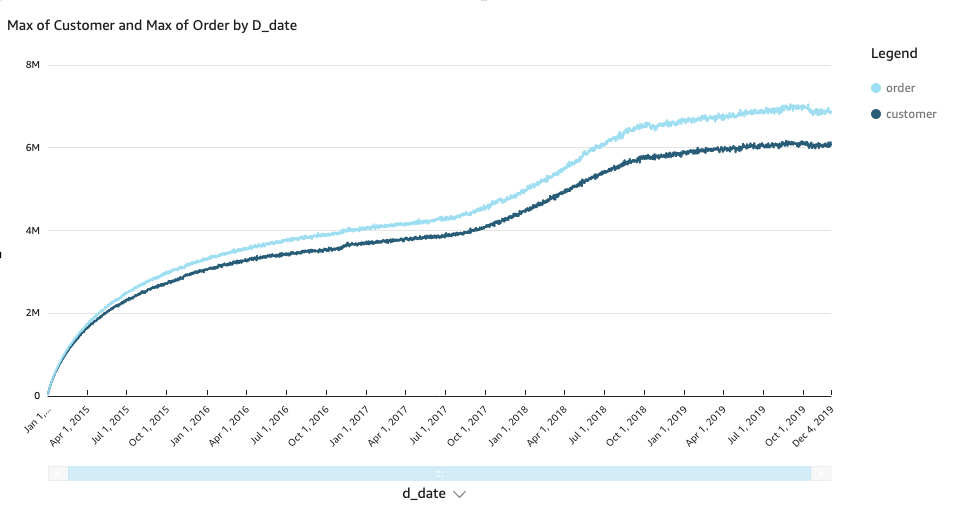
Now the data is ready to be analyzed. Let’s look at the overall customer trend in the past 5 years. The following query takes less than 5 seconds using HLL sketches, which makes interactive analysis easy:
SELECT d_date,
       Hll_cardinality(Hll_combine(hll_customer)) AS customer,
       Hll_cardinality(Hll_combine(hll_order))    AS order
FROM   sales_sketch
GROUP  BY d_date;

Runtime: 4.9 seconds
The same analysis using COUNT DISTINCT uses more resources and takes several minutes, and query runtime also grows linearly with data growth.
The following visualization of our result shows that our sales grew in a steady upward trend. In the last 2 years, the growth increased faster.
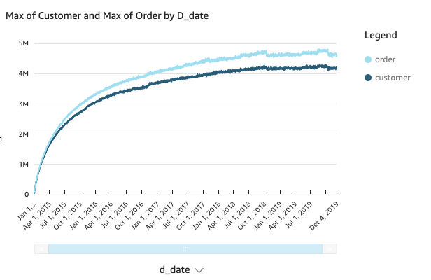
Let’s drill down to each sales channel and find out what action triggered it.
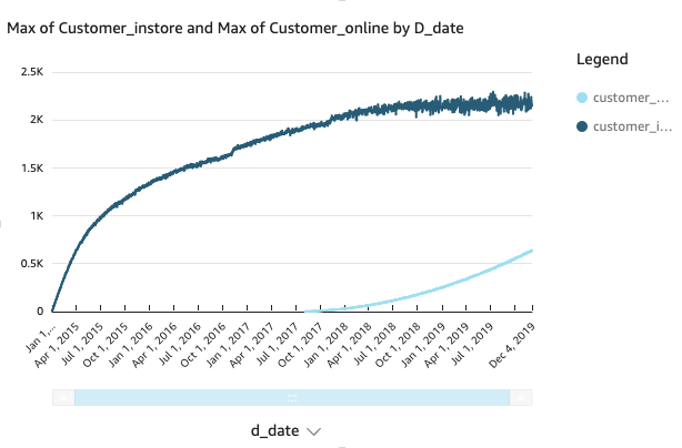
We can see it’s due to the online sales we added from that time. Adding the online channel is definitely a great strategy.
SELECT   d_date,
         Hll_cardinality(Hll_combine(hll_customer)) AS customer,
         Hll_cardinality(Hll_combine(hll_order))    AS ORDER
from     sales_sketch
WHERE    channel = 1
GROUP BY d_date;

Runtime: 2.92 seconds

SELECT   d_date,
         Hll_cardinality(Hll_combine(hll_customer)) AS customer,
         Hll_cardinality(Hll_combine(hll_order))    AS ORDER
from     sales_sketch
WHERE    channel = 2
GROUP BY d_date;

Runtime: 2.96 seconds
The following visualization shows the in-store results
The following visualization shows the online results.

With the fine-grained HLL sketch computed, we can filter or group by any combination of date range, sales channel, and product, then merge the HLL sketch to get a final approximate distinct count. Now let’s compare the top 10 popular products per sales channel:
SELECT   product,
         Hll_cardinality(Hll_combine(hll_customer)) AS instore
FROM     sales_sketch
WHERE    channel = 1
GROUP BY product
ORDER BY instore DESC limit 10;
SELECT   product,
         Hll_cardinality(Hll_combine(hll_customer)) AS online
FROM     sales_sketch
WHERE    channel = 2
GROUP BY product
ORDER BY online DESC limit 10;
Regardless of if we use a channel filter or not, all queries have consistent fast performance under 2 seconds.
The following table shows that the top 10 in-store products are completely different from the online products.
| instore | online |
| 1001 | 599 |
| 1501 | 749 |
| 2003 | 445 |
| 501 | 149 |
| 1251 | 743 |
| 1505 | 899 |
| 2251 | 437 |
| 2009 | 587 |
| 5 | 889 |
| 3 | 289 |
Let’s dig into a few products and compare sales channel performance:
WITH instore
     AS (SELECT d_date,
                Hll_cardinality(Hll_combine(hll_customer)) AS customer_instore
         FROM   sales_sketch
         WHERE  product = <product_id> AND channel = 1
         GROUP  BY d_date),
     online
     AS (SELECT d_date,
                Hll_cardinality(Hll_combine(hll_customer)) AS customer_online
         FROM   sales_sketch
         WHERE  product = <product_id> AND channel = 2
         GROUP  BY d_date)
SELECT instore. d_date,
       customer_instore,
       customer_online
FROM   instore
       LEFT OUTER JOIN online
                    ON instore.d_date = online. d_date
ORDER BY instore. d_date;

Runtime 0.5s
The following visualization shows the Product 1 results.
The following visualization shows the Product 2 results.
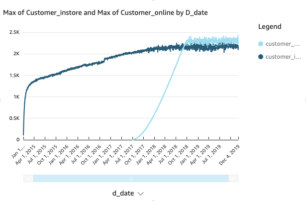
In the preceding example, Product 1 wasn’t as popular with customers online as Product 2. This informs inventory planning in the distribution centers as well as the retail stores to increase sales.
Lastly, let’s analyze seasonal product performance. For seasonal items, the turnover rate is much quicker, so we want to monitor the trend more closely and make adjustments as soon as possible.
The following code monitors the performance of our top seasonal product:
WITH top_1_product as (
              SELECT   product
              FROM     sales_sketch
              WHERE    channel = 3
              GROUP BY product
              ORDER BY Hll_cardinality(Hll_combine(hll_order)) DESC
              limit 1)
SELECT   d_date,
         Hll_cardinality(Hll_combine(hll_customer)) AS customer
FROM     sales_sketch
WHERE    product IN (select product from top_1_product)
AND      channel = 3
GROUP BY d_date;

Runtime 2.7s
The following visualization shows our results.

To get a full picture quickly, we can compute the latest sales data on the fly and merge it with the HLL sketch history to get a complete result:
WITH full_sales AS
(
         SELECT   product,
                  d_date,
                  Hll_create_sketch(customer)     AS hll_customer,
                  Hll_create_sketch(order_number) AS hll_order
         FROM     seasonal_sales
         WHERE    d_date = <CURRENT_DATE>
         GROUP BY product,
                  d_date
         UNION ALL
         SELECT product,
                d_date,
                hll_customer,
                hll_order
         FROM   sales_sketch
         WHERE  channel = 3)
SELECT   product,
         hll_cardinality(hll_combine(hll_customer)) AS seasonal
FROM     full_sales
GROUP BY 1
ORDER BY 2 DESC;

Runtime 0.9s
The HLL sketch provides you flexibility and high performance, and enables interactive trend analysis and near-real-time trend monitoring. For hot data like recent 1-week data, we can even keep hourly granularity. After 1 month, we can roll the daily sketch data up to monthly to get even better performance.
Conclusion
You can use HyperLogLog for a lot of use cases. For a video demo of another use case, check out Amazon Redshift HyperLogLog Demo.
Evaluate your use cases to see if they can use approximate count and take advantage of the HLL capability of Amazon Redshift.
About the Author
Juan Yu is an Analytics Specialist Solutions Architect at Amazon Web Services, where she helps customers adopt cloud data warehouses and solve analytic challenges at scale. Prior to AWS, she had fun building and enhancing MPP query engines to improve customer experience on Big Data workloads.
Costas Zarifis is a Software Development Engineer at AWS. He spends most of his time building cutting-edge features for the Redshift cloud infrastructure and he is the lead developer of the HLL type and functionality in Redshift. He is passionate about learning new and exciting technologies, and enjoys working on large scalable systems. Costas holds a Ph.D. from the University of California, San Diego and his interests lie in web and database application frameworks and systems.
Enjoyed this article? Sign up for our newsletter to receive regular insights and stay connected.