Revolutionize Your Factor Investing with Machine Learning

Zero to one in Financial ML Developer with SKlearn

Factor investing has gained significant popularity in the field of modern portfolio management. It refers to a systematic investment approach that focuses on specific risk factors or investment characteristics, such as value, size, momentum, and quality, to construct portfolios. The blossoming of machine learning in factor investing has its source at the confluence of three favorable developments: data availability, computational capacity, and economic groundings. So this article will discuss Factor Investing with Machine Learning.

Basic Knowledge of Factor Investing

Factor investing has gained significant popularity in the field of modern portfolio management. It refers to a systematic investment approach that focuses on specific risk factors or investment characteristics, such as value, size, momentum, and quality, to construct portfolios. These factors are believed to have historically exhibited persistent risk premia that can be exploited to achieve better risk-adjusted returns.

The historical roots of factor investing can be traced back to several decades ago. In the 1960s, pioneering academics like Eugene F. Fama and Kenneth R. French conducted groundbreaking research that laid the foundation for modern factor investing. They identified specific risk factors that could explain the variation in stock returns, such as the value factor (stocks with low price-to-book ratios tend to outperform), the size factor (small-cap stocks tend to outperform large-cap stocks), and the momentum factor (stocks with recent positive price trends tend to continue outperforming).

By incorporating factor-based strategies into their portfolios, investors can aim to achieve enhanced diversification, improved risk-adjusted returns, and better risk management. Factor investing provides an alternative approach to traditional market-cap-weighted strategies, allowing investors to potentially capture excess returns by focusing on specific risk factors that have demonstrated historical performance.

The main reason why Factor Investing is so popular may be because Factor Investing can be easily explained in investment management.

Step to Step with sklearn

In my last article, I talk about Financial Machine Learning with Scikit-Learn and use “200+ Financial Indicators of US stocks (2014–2018)” dataset from Kaggle. In this article, I will use the same dataset. So, You can view details from my last article.

The common procedure and the one used in Fama and French (1992). The idea is simple. On one date,

1. rank firms according to a particular criterion
2. Form J≥2 J≥2 portfolios (i.e., homogeneous groups) consisting of the same number of stocks according to the ranking (This article use medium)

We will start with a simple factor, Size Factor. We will cluster stocks into two groups Big/Small, We’ll see if size can generate alpha.

# Define a variable for filtering
filter_value = df_2014[["Market Cap"]].median()[0]

# Filter rows based on the variable
Big_Cap = df_2014[df_2014['Market Cap'] > filter_value]
Small_Cap = df_2014[df_2014['Market Cap'] < filter_value]

print("Big cap alpha", Big_Cap["Alpha"].mean())
print("Small cap alpha", Small_Cap["Alpha"].mean())

We can see that in 2014 Big cap have alpha 3.91, Small cap stocks -3.28.

Let’s look at some other years.

Year_lst = ["2014", "2015", "2016", "2017", "2018"] 
dic_alpha_bigcap = {}

for Year in Year_lst :

    data =   df_all[df_all['Year'] == Year]
    filter_value = data[["Market Cap"]].median()[0]
    Big_Cap = data[data['Market Cap'] > filter_value]

    print("Year : ", Year )
    print("Big cap alpha", Big_Cap["Alpha"].mean())

    dic_alpha_bigcap [Year] = Big_Cap["Alpha"].mean()

Year_lst = ["2014", "2015", "2016", "2017", "2018"] 
dic_alpha_Small_Cap = {}

for Year in Year_lst :

    data =   df_all[df_all['Year'] == Year]
    filter_value = data[["Market Cap"]].median()[0]
    Small_Cap = data[data['Market Cap'] < filter_value]

    print("Year : ", Year )
    print("Small cap alpha", Small_Cap["Alpha"].mean())

    dic_alpha_Small_Cap [Year] = Small_Cap["Alpha"].mean()

At this point, we may conclude that the year 2014 -2019 Big cap. perform more Small cap.We will do this for all variables.

def filter_data_top (column,df_all ) :

    Year_lst = ["2014", "2015", "2016", "2017", "2018"] 
    dic_alpha = {}

    for Year in Year_lst :
        data =   df_all[df_all['Year'] == Year]
        filter_value = data[[column]].median()[0]
                            
        filterdata = data[data[column] > filter_value]                   
        
        print("Year : ", Year )
        print(column, filterdata["Alpha"].mean())
        
        dic_alpha[Year] = filterdata["Alpha"].mean()

    return dic_alpha

def filter_data_below (column,df_all ) :

    Year_lst = ["2014", "2015", "2016", "2017", "2018"] 
    dic_alpha = {}

    for Year in Year_lst :
        data =   df_all[df_all['Year'] == Year]
        filter_value = data[[column]].median()[0]
                            
        filterdata = data[data[column] < filter_value]                   
        
        print("Year : ", Year )
        print(column, filterdata["Alpha"].mean())
        
        dic_alpha[Year] = filterdata["Alpha"].mean()

    return dic_alpha

lst_alpha_all_top = []

for factor in df_all.columns[2:] :
    try:        
        print(factor)
        dic_alpha = filter_data_top (column= factor,df_all = df_all)
        
        df__alpha = pd.DataFrame.from_dict(dic_alpha, orient='index',columns=[factor])
        lst_alpha_all_top.append(df__alpha)
    
    except:
        print("error")

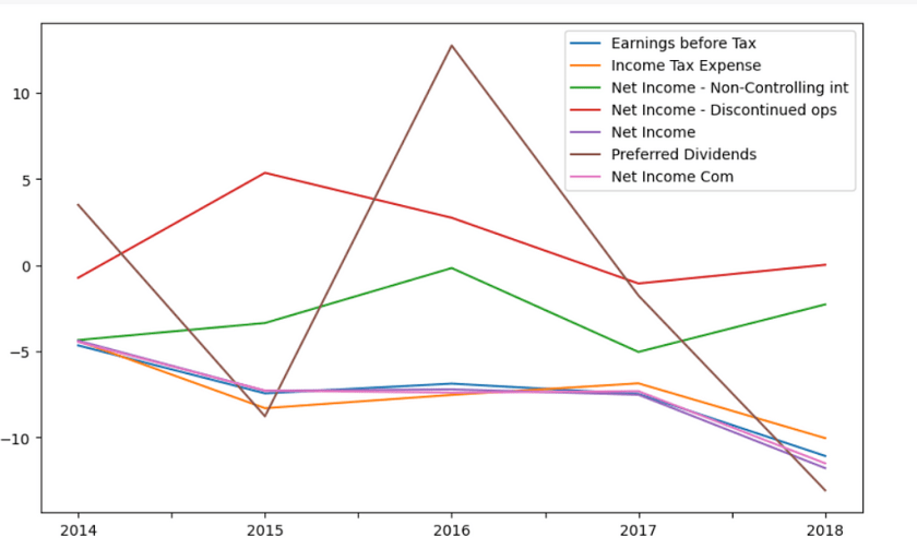
Finally, we get a alpha table.

You can plot.

df_below_alpha.iloc[:,8:15].plot(figsize= (10, 6))
plt.legend(loc = "best");

The Big Question What’s Factor Can Generate Alpha?

When analyzing stock returns, if we assume that all returns of all stocks are stacked in a vector ‘r’, and ‘x’ is a lagged variable that exhibits predictive power in a regression analysis, it may be tempting to conclude that ‘x’ is a good predictor of returns if the estimated coefficient ‘b-hat’ is statistically significant based on a specified threshold. To test the importance of ‘x’ as a factor in predicting returns, we can use Factor Importance Tests, where ‘x’ is treated as the factor and ‘y’ is the alpha. In the Fama and French equation, ‘y’ is typically represented as ‘Return’, but it can also be interpreted as ‘Return minus Ri and Ri-Rf’, which is essentially the alpha. While we won’t delve into the details of this section here, you can refer to the article at this if you are interested in learning more about this topic.”

Note : We need to change the variable to percentile

Year_lst = ["2014", "2015", "2016", "2017", "2018"] 
dic_rank  = {}

for Year in Year_lst :

    data =   df_all[df_all['Year'] == Year]
    df_rank = df_all.rank(pct=True)

    dic_rank[Year] = df_rank
df_rank = pd.concat(dic_rank)

I’ll introduce another technic call “Maximal Information Coefficient” Maximal Information Coefficient (MIC) is a statistical measure that quantifies the strength and non-linearity of association between two variables. It is used to assess the relationship between two variables and determine if there is any significant mutual information or dependence between them. MIC is particularly useful in cases where the relationship between two variables is not linear, as it can capture non-linear associations that may be missed by linear methods such as correlation.

MIC is considered important because it offers several advantages:

1. Captures Non-Linear Associations: Unlike linear correlation, which only measures linear relationships, MIC can capture non-linear associations between variables. This makes it useful in scenarios where the relationship between variables may not be well-described by a linear relationship.
2. Measures Both Strength and Non-Linearity: MIC combines measures of both strength and non-linearity of association, providing a holistic assessment of the relationship between variables. This allows it to detect complex patterns of dependence, including both linear and non-linear relationships.
3. Robust to Noise and Scale: MIC is robust to noise and scale differences between variables, making it suitable for analyzing data with varying levels of noise or measurement errors.
4. Provides a Normalized Value: MIC is normalized to a value between 0 and 1, where 0 indicates no association and 1 indicates a perfect association. This makes it easy to interpret and compare the strength of associations across different datasets or variables.
5. Applications in Various Fields: MIC has been widely used in various fields such as finance, bioinformatics, ecology, and social sciences, among others. It has found applications in feature selection, dimensionality reduction, and identifying complex patterns in large datasets.

We use minepy for test MIC.

X_ = X["Revenue Growth"]
y = df_all["Alpha"]

mine = MINE( est="mic_approx")
mine.compute_score(X_, y)
mine.mic()

How to use ML to improve Factor Investing

We have previously explained how factor investing works. Machine learning (ML) techniques can be used to improve factor investing in various ways. ML algorithms can help identify relevant factors with predictive power, optimize the combination of factors, determine the optimal timing of factor exposures, enhance risk management, optimize portfolio construction, and incorporate alternative data sources. By analyzing historical data and applying ML algorithms, investors can identify factors, optimize their combination, and dynamically adjust exposures based on market conditions. ML techniques can also enhance risk management measures and incorporate alternative data for better insights.

We use linear regression using the LinearRegression class from the sklearn.linear_model module in Python. The goal is to fit a linear regression model to the data in df_rank DataFrame to predict the values of the dependent variable, denoted as y, using the values of the independent variable, denoted as X, which is derived from the “PE ratio” column of df_rank.

Import LinearRegression

from sklearn.linear_model import LinearRegression

This line imports the LinearRegression class from the sklearn.linear_model module, which provides implementation of linear regression in scikit-learn, a popular machine learning library in Python.

Define the dependent variable:

y = df_all["Alpha"]

This line assigns the “Alpha” column of df_all DataFrame to the variable y, which represents the dependent variable in the linear regression model.

X = df_rank[["PE ratio"]].fillna(value=df_rank["PE ratio"].mean())

This line assigns a DataFrame containing the “PE ratio” column of df_rank DataFrame to the variable X, which represents the independent variable in the linear regression model. The fillna() method is used to fill any missing values in the “PE ratio” column with the mean value of the column.

PElin_reg = LinearRegression()

This line creates an instance of the LinearRegression class and assigns it to the variable PElin_reg.

Fit the linear regression model:

PElin_reg.fit(X, y)

This line fits the linear regression model to the data, using the values of X as the independent variable and y as the dependent variable.

Extract the model coefficients:

PElin_reg.intercept_, PElin_reg.coef_

These lines extract the intercept and coefficient(s) of the linear regression model, which represent the estimated parameters of the model. The intercept is accessed using the intercept_ attribute, and the coefficient(s) are accessed using the coef_ attribute. These values can provide insights into the relationship between the independent variable(s) and the dependent variable in the linear regression model.

Repeat with ROE

from sklearn.linear_model import LinearRegression
y = df_all["Alpha"]
X = df_rank[["ROE"]].fillna(value=df_rank["ROE"].mean() )


ROElin_reg = LinearRegression()
ROElin_reg.fit(X, y)
ROElin_reg.intercept_, ROElin_reg.coef_

And plot

import matplotlib.pyplot as plt

X1 = df_rank[["PE ratio"]].fillna(value=df_rank["PE ratio"].mean() )
X2 = df_rank[["ROE"]].fillna(value=df_rank["ROE"].mean() )

plt.figure(figsize=(6, 4))  # extra code – not needed, just formatting
plt.plot( X1, PElin_reg.predict(X1), "r-", label="PE")
plt.plot(X2  , ROElin_reg.predict(X2) , "b-", label="ROE")

# extra code – beautifies and saves Figure 4–2
plt.xlabel("$x_1

quot;)
plt.ylabel("$y

quot;, rotation=0)
# plt.axis([1, 1, ])
plt.grid()
plt.legend(loc="upper left")

plt.show()

We can see that the PE line has a higher slope( coef_). Therefore, we can say that PE can predict an Alpha value.If we have 3 stocks and we want to know which one will perform.

Here we will try to predict Alpha’s rank from 10 variables.

y = df_all["Alpha"]
X = df_rank.fillna(value=df_rank.mean() )
bestfeatures = SelectKBest(k=10, score_func=f_regression)
fit = bestfeatures.fit(X,y)

repeat

from sklearn.linear_model import LinearRegression

top_fest = featureScores.nlargest(10,'Score')["Specs"].tolist()

y = df_rank["Alpha"]
X = df_rank[top_fest].fillna(value=df_rank[top_fest].mean() )


lin_reg = LinearRegression()
lin_reg.fit(X, y)

lin_reg.predict(X)

Handle data

df_ =  df_all[["Unnamed: 0", "Sector", "Year"]]
df_["Alpha_rank"] = df_rank["Alpha"]
df_["Predict_Alpha"] = lin_reg.predict(X)

print MSE

from sklearn.metrics import mean_squared_error
X = df_["Unnamed: 0"]
Y1 = df_["Alpha_rank"]
Y2 = df_["Predict_Alpha_rank"]

mean_squared_error(Y1, Y2)

MSE = 0.07 , it indicates that, on average, the squared differences between the predicted values and the actual values (i.e., the residuals) are relatively small. A lower MSE generally indicates better model performance, as it signifies that the model’s predictions are closer to the actual values.

But,

import matplotlib.pyplot as plt

X = df_["Unnamed: 0"].head(30)
Y1 = df_["Alpha_rank"].head(30)
Y2 = df_["Predict_Alpha"].head(30)

plt.figure(figsize=(6, 6))  # extra code – not needed, just formatting
plt.plot( X, Y1, "r.", label="Alpha")
plt.plot( X , Y2 , "b.", label="Predict_Alpha")

# extra code – beautifies and saves Figure 4–2
plt.xlabel("$x_1

quot;)
plt.ylabel("$y

quot;, rotation=0)
# plt.axis([1, 1, ])
plt.grid()
plt.legend(loc="upper left")

plt.show()

We can see that, Although MSE it’s less but, We can see that the predicted value is in the middle. That is because of the limitations of the Liner regression model.

Computational Complexity

Now we will look at a very different way to train a linear regression model, which is better suited for cases where there are a large number of features or too many training instances to fit in memory.

Gradient Descent

Gradient descent is an optimization algorithm commonly used in machine learning to minimize a loss or cost function during the training process of a model. It is an iterative optimization algorithm that adjusts the model parameters in the direction of the negative gradient of the cost function in order to find the optimal values for the parameters that minimize the cost function.

from sklearn.linear_model import SGDRegressor

sgd_reg = SGDRegressor(max_iter=100000, tol=1e-5, penalty=None, eta0=0.01,
                       n_iter_no_change=100, random_state=42)
sgd_reg.fit(X, y.ravel())  # y.ravel() because fit() expects 1D targets

Learning Curves

Sometimes we have too many variables. We want to fit training data much better than plain linear regression.This case we use 100 variables. We use learning_curve function to help us.

from sklearn.model_selection import learning_curve

train_sizes, train_scores, valid_scores = learning_curve(
    LinearRegression(), X, y, train_sizes=np.linspace(0.01, 1.0, 40), cv=5,
    scoring="neg_root_mean_squared_error")
train_errors = -train_scores.mean(axis=1)
valid_errors = -valid_scores.mean(axis=1)

plt.figure(figsize=(6, 4))  # extra code – not needed, just formatting
plt.plot(train_sizes, train_errors, "r-+", linewidth=2, label="train")
plt.plot(train_sizes, valid_errors, "b-", linewidth=3, label="valid")

# extra code – beautifies and saves Figure 4–15
plt.xlabel("Training set size")
plt.ylabel("RMSE")
plt.grid()
plt.legend(loc="upper right")
#plt.axis([0, 80, 0, 2.5])

plt.show()

The optimal Training set size data is the red line close to the blue line. If the red line is much lower than the blue line, it is called Underfit. On the other hand, If the red line is much upper than the blue line Overfit.

Beyond ……………………

At this point, we will get the coefficient. The coefficient can tell what factors determine returns.We still have a lot of details that we skipped(Normalization, Factor engineering, etc.)Other algorithms(Regularized Linear Models,Lasso Regression,Elastic Net) and Including the use of ML in various steps.

Ref :

Machine Learning for Factor Investing by Guillaume Coqueret

1. “Advances in Financial Machine Learning” by Marcos Lopez de Prado: This book provides an in-depth overview of the intersection of finance and machine learning, including techniques for factor modeling, risk management, and portfolio optimization using machine learning algorithms.
2. “Machine Learning for Factor Investing: Empirical Methods for Systematic Trading” by Marcos Lopez de Prado:
3. “Applied Machine Learning” by Kelleher, Mac Namee, and D’Arcy
4. “Quantitative Momentum: A Practitioner’s Guide to Building a Momentum-Based Stock Selection System” by Wesley R. Gray and Jack R. Vogel
5. Hands-on ml with scikit-learn keras and tensorflow by Geron Aurelien
6. Machine Learning and Data Science Blueprints for Finance: From Building Trading Strategies to Robo-Advisors Using Python by Hariom Tatsat , Sahil Puri , Brad Lookabaugh

Note Book

Google Colaboratory

Subscribe to DDIntel Here.

Visit our website here: https://www.datadriveninvestor.com

Join our network here: https://datadriveninvestor.com/collaborate

---

Revolutionize Your Factor Investing with Machine Learning was originally published in DataDrivenInvestor on Medium, where people are continuing the conversation by highlighting and responding to this story.